How To Freeze the Top Row in Excel

If you regularly work with large spreadsheets, you know the convenience of headers and categories, especially when you scroll down through the spreadsheet’s rows. Losing those headings can make data more difficult to interpret. Freezing the top row in Excel preserves those precious headings/categories as you move down your spreadsheet. You won’t have to memorize the categories anymore.

The feature is called Freeze Panes, and it holds the first row or the first column in place while you scroll through the spreadsheet. The setting makes comparing data much easier and helps prevent errors, especially those that involve data insertion. Placing data in the wrong cell can have major repercussions.

Here’s how to lock the top row in Excel 2007, 2010, 2016, 2019, and Office 365.

1. Open the Worksheet you want to work on.
   
2. Select the “View” tab and navigate to “Freeze Panes.”
   
3. Select “Freeze Top Row.”
   

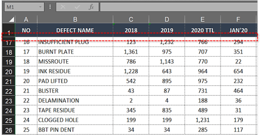
You should now see the top row become bordered with a thin box. Scrolling down the page will keep the top row in place for the entirety of the spreadsheet.

Freeze Multiple Rows in Excel

If your headings take up more than a single row or you want to compare data in a couple of the top rows to elsewhere in the spreadsheet, you can freeze multiple rows in a similar way.

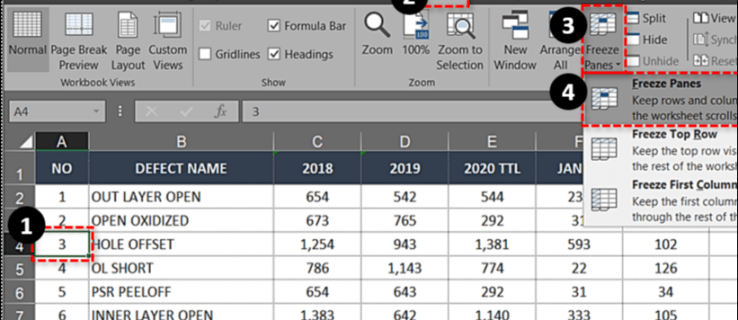
1. Click on the first cell in the column below the rows you want to freeze.
   
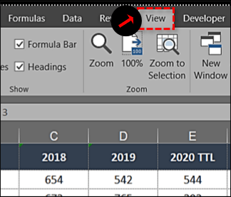
2. Select the “View” tab.
   
3. Click the “Freeze Panes” box, then choose “Freeze Panes” from the list.
   

The above steps should lock the selected, adjacent top rows so you can scroll down and keep the headings in place while doing it.

For example, if you want to freeze the top three rows of a Worksheet, you would select the first cell in A4. Once you freeze the panes, lines A1, A2, and A3 would be frozen and you can scroll wherever you need to compare the data.

Freeze a Column in Excel

Freezing a column has similar uses in Excel. If your spreadsheet has multiple columns that require scrolling across the page, locking the first column down can help make sense of all that data.

1. Open the Worksheet you want to work on.
2. Select the View tab and navigate to Freeze Panes.
3. Select Freeze First Column.

You use the same tools as freezing rows but make a different selection within the dropdown.

Freeze Multiple Columns in Excel

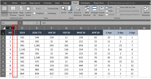
If you want to freeze multiple columns in Excel, you do that in the same way as you would freeze multiple rows.

1. Select the column to the right of the column you want to freeze.
2. Select the View tab and Freeze Panes.
3. Select Freeze Panes.

For example, if you wanted to freeze the first three columns, select column D and Freeze Panes. Columns A, B and C will then be frozen. You can also select cell D1 to achieve the same thing.

Freeze Columns and Rows in Excel

You can also freeze columns and rows in Excel to make short work of data comparison.

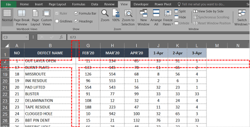
1. Select the cell one row below and one column right of the rows and columns you want to freeze.
2. Select Freeze Panes and Freeze Panes again.

For example, if you wanted to freeze columns A and B and rows 1 and 2, you would select cell C3. Freeze panes will lock down the first two columns and rows until you unfreeze them.

Unfreeze Rows or Columns in Excel

If you just need to freeze a row temporarily to compare data, you can unfreeze once you’re done. It does not affect any data or the formatting so it would be as if you had never done it.

1. Select the View tab and Freeze Panes.
2. Select Unfreeze Panes.

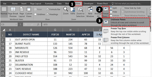
It doesn’t matter whether you froze the first row, multiple rows, first column or multiple columns, this setting removes it.

Freezing Rows and Columns Issues in Excel

If you cannot freeze a row or a column in Excel, it could be that you are in cell editing mode. If you have been writing or modifying a formula, the Freeze Pane selection may be grayed out. Hit Esc to exit cell editing mode and you should be able to select Freeze Pane as normal.

If you are trying to freeze a spreadsheet you didn’t create, it may be protected. That should be identifiable by the little padlock or the fact you may not be able to save it. Select File from the top menu, then Protect Workbook and select Unprotect. You can also do this within a sheet by selecting the Review tab and Unprotect Sheet in the Ribbon.

Let's block ads! (Why?)