How to Show the Current Time in a Google Sheet

One of the many functions Google Sheets users can perform in the app is to show the current time. First-time users may be confused with the syntax at first, but fortunately, displaying time in your spreadsheet is a relatively straightforward process.

In this article, we’ll show you how to use these functions to show current time using the two most popular functions: NOW and TIME. Whether you want to display both date and time or just one value, these functions have got you covered. You’ll also learn how to customize the results so you can get the most out of this handy feature.

How to Show the Current Time in a Google Sheet?

Showing current time in a Google Sheet is a feature many users, especially data analysts, use to keep the activity log of different operations. The date and time functions work by retrieving the time from your computer straight into a spreadsheet cell you select as active.

Below, you’ll find detailed instructions on how to show current time using the most common functions.

Adding the Current Time and Date Using NOW

Let’s start with one of the most widely used functions to show the current date. You can use this formula to add the current date (or time) onto your spreadsheet or incorporate it into a different date or time formula.

The syntax for the NOW function is as follows:

=NOW()

This syntax consists of the name, brackets, and comma separators. It doesn’t have any arguments that are usually a part of the syntax and are entered inside the brackets.

If you do bookkeeping or perform other tasks that need you to add the exact date and time on a specific spreadsheet, it’s best to use the NOW function.

1. Open a Google spreadsheet or create a new one.
2. Click on a cell in which you want to display the current date and time. This will make the cell active.
3. Type “=NOW() “and press enter. The brackets make sure you’re using this word as a function. You’ll now see the date and time appear in the cell where you’ve entered the formula. You can see the complete function in the bar on top of the worksheet.
   

Here’s what you should know about the NOW function:

• The NOW function is volatile. It recalculates or updates every time its spreadsheets are edited. In the spreadsheet settings, you can choose to recalculate the worksheet “On change and every minute” or “On change and every hour.” However, there is no way to turn off volatile function recalculations.
• The date and time showing in the spreadsheet will always refer to the current time after recalculating the spreadsheet and not the date and time of its first entry.
• You can change the number formatting to hide one component of the function.

How to Insert Current Date Using TODAY?

To only display the current date in Google Sheets without the time stamp, it’s best to use the TODAY function. Depending on your local settings, the date will show in the DD/MM/YY or the MM/DD/YY format. Similar to the NOW function, TODAY doesn’t have any arguments. This means there will be no syntax between the brackets.

Follow the steps below to insert the current date using the TODAY function:

1. Select an empty cell from your Google Sheet to make it active.
2. Type “=TODAY()” and press enter.
   

The cells containing the TODAY formula update each day, and you can further customize the formatting to use numbers or text according to your preference.

Formatting Your Formulas

By default, the NOW function shows a time and date timestamp on your Google Sheet. To change this setting, you need to tweak the formatting for the cell that contains that timestamp. Also, the same formatting rules go for the TODAY formula as well.

Follow the steps below to change the formatting of your formulas:

1. Select the cell showing the time and date with the NOW (or TODAY) formula.
2. Click on “Format” from the toolbar above the spreadsheet.
   
3. Hover over the “Number” option from the drop-down menu.
   
4. Select “Time” if you want the function only to show the current time. Likewise, select “Date” for the function to only display the current date.
   

If you want to modify the NOW or TODAY function format, you can do so from the Format menu by following the steps below:

1. Select the cell you wish to modify. You can select a range of cells as well.
2. Click on “Format,” then “Number,” and “More Formats.” Next, look for the “More Date and Time Formats” option, which will open a new dialog box.
   
3. You can choose from more than a dozen formats. Select the one you want and click on the “Apply” button in the upper right-hand of the dialog box. The date can be written in the form of numbers, include text, or have additional characters (forward slash).
   
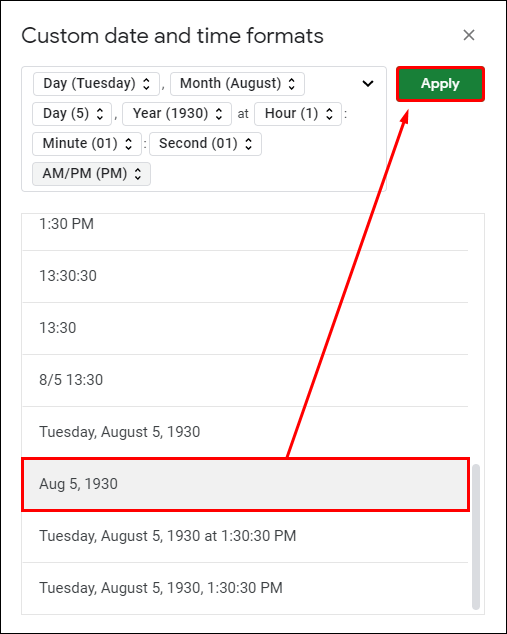
4. Go back to the cells to check whether they match the format you set.
   

You can apply various formats for different cells on your Google Sheet.

Additional FAQs

How to Insert Static Times or Dates in Google Sheet?

If you prefer to work with static date and time, you can use a shortcut option that includes either manually writing the date and time or entering them using the following commands:

• “Ctrl +;” – static date shortcut (Windows)

• “Ctrl + Shift + :” – static time and date shortcut (Windows)

• “Command + ;” – static time shortcut (Mac)

The NOW and TODAY formulas can’t display static times.

Adding the Current Time and Date Using GoogleClock

Adding current time and date using GoogleClock is not supported anymore. This function was used for spreadsheets that were published on the web and only occasionally updated. Instead of GoogleClock, you can use the NOW or TODAY formulas to add current time and date into your Google Spreadsheet.

How to Convert Time to Decimal in Google Sheets?

Chances are, you may have to convert the time and date data values in your Sheet into decimals. This conversion is often present when converting the difference between the beginning and end times of a task into decimals.

To convert time to decimal numbers in Google Sheets, you can use the time functions such as HOUR, MINUTE, or SECOND, or the TIMEVALUE function.

The HOUR Function

The hour function will take in a specific time value and return only its hour component. So, for the time value of “05:14:40,” it will return ‘’5’’ as it rounds to the nearest hour.

Here’s the function syntax:

=HOUR(time)

In this function, “time” shows a time value or a reference to a cell with a time value.

The MINUTE Function

This function does the same thing as the previous one but only returns the minute value. For the same time value of “15:14:40,” it will return ‘’15.’’

Here is the syntax:

=MINUTE(time)

The SECOND Function

Like the HOUR and the MINUTE function, the SECOND function will return the second component of a cell’s time value. So, if we take the same example, “15:14:40,” the function will return ‘’40.’’

The syntax is as follows:

=SECOND(time)

Converting Time to the Number of Hours

When you have the hour, minute, and the second number in a time value, you can also convert it to a decimal that’s equivalent to that value in terms of hours by using the formula below:

=HOUR(B3)+MINUTE(B3)/60+SECOND(B3)/3600

B3 in this example refers to the cell where the time value is active. It can be any cell you select on your spreadsheet.

Convert Time to Number of Minutes

You can follow the same logic to convert a time value to the decimal equivalent to the number of minutes.

=HOUR(B3)*60+MINUTE(B3)+SECOND(B3)/60

Again, the B3 here is only an illustration.

Convert Time to Number of Seconds

=HOUR(B3)*3600+MINUTE(B3)*60+SECOND(B3)

This is the formula you should apply to convert time from the cell containing the time value (we assume it’s B3) to a number of seconds.

How to Calculate Times in Google Sheet?

If you work with spreadsheets often, you’re likely to calculate the time difference between two events or timestamps. To calculate that difference, the cells with the time data need to be formatted as such. Otherwise, Google Sheets won’t recognize them, and the difference between 8:00 AM and 10:00 AM will be calculated as 200, rather than two hours.

Here’s how to set up your spreadsheet, so it’s properly formatted:

1. Open the Google Spreadsheet you need to work on.

2. Select the start time column and click on the “123” option from the toolbar.

3. Select “Time” from the drop-down menu.

4. Repeat steps 2 and 3 for the second column (end time).

All you need to do now is use the formula that subtracts the Start time column from the End time column. You’ll receive the time that has elapsed between these cells displayed as hours.

If the start time is in column A and end time in B, you can click on a cell from the column C and type in the following syntax:

=B2-A2

Another way to calculate time in Sheets is via the TEXT function:

=TEXT (B3-A3, “h”) – to calculate hours

=TEXT(B3-A3, “h:mm”) – to calculate hours and minutes

=TEXT(B3-A3, “h:mm:ss”) – to calculate hours, minutes, and seconds

Time Waits for No One

Showing current time and date in Google Sheets is a simple operation everyone can perform with a little help. This article provided you with all the necessary instructions to seamlessly show all time and date values you need, format them or convert them to decimal numbers.

Whether you’re a financial or data analyst or you simply work on spreadsheets often, you’ll never have to worry about displaying time and date on your sheets again.

For which operations do you use the NOW and TODAY formulas? Do you prefer to keep the default number formatting or change it to a more specific one? Share your experiences in the comments section below.

Adblock test (Why?)

Original page link

Best Cool Tech Gadgets

Top favorite technology gadgets