How To Sum a Row in Google Sheets

Google Sheets offers plenty of tools to simplify complicated calculations, one of them being the SUM function. While it’s a basic formula, not every Google Sheets user knows about all the benefits of using it. Furthermore, the way you enter the formula and values may affect how the function works.

If you’re wondering how to sum an entire row in the app correctly, we’re here to help. In this guide, we’ll explain how to sum a row in Google Sheets the right way. We’ll also share instructions on how to add up only selected values or a range of cells. Additionally, we’ll answer some questions related to the topic.

SUM Functions in Google Sheets

The SUM function in Google Sheets, just as in Microsoft Office Excel, sums selected values. It’s helpful because it may be too much of a hassle to enter a formula if you only need to add up a few values. Sure, you can find “2+3+4” without the help of a computer. But in practice, the formula is extremely useful for any values.

The main benefit is that the sum updates automatically when any of the values are changed or added to a selected row or column. For instance, if you change “2” in the above-mentioned example to “1,” the value in the sum cell will update from “9” to “8” on its own.

On the other hand, without the formula, you’d have to recalculate the sum every time you make changes. For this reason, we advise you not to enter the value itself when using the “=SUM” formula. Instead, type in the number of a cell containing the value. We’ll take a closer look at how to use the function in the next section.

How to Enter the Formula

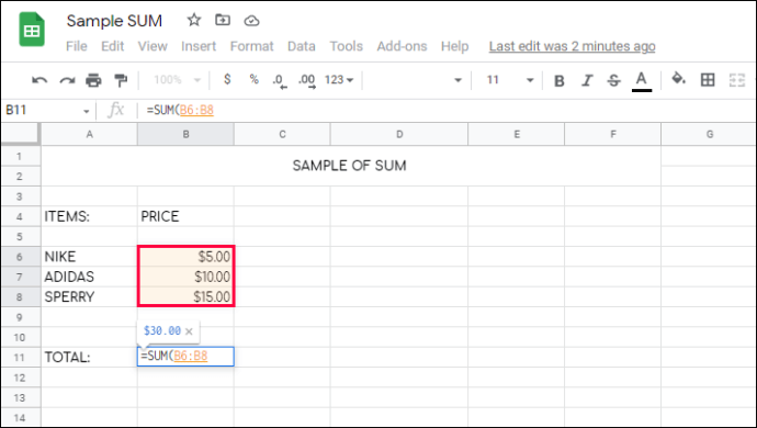
Now that you know why the SUM function is so useful, it’s time to find out how to use it. To sum an entire row, follow the instructions below:

1. Click any blank cell.
   
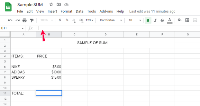
2. At the bottom of your screen, click “Enter text or formula” and type in “=SUM(”.
   
3. To sum a total row, click the number to the left from your row, for instance, “1.”
   
4. Hit the “Enter” key or click the green checkmark to the left from your formula. The result will appear in your selected cell.
   

Note: When you select a whole row by clicking the number at the left, new values entered into this row are automatically added to the sum.

If you wish to only select certain cells, here’s the first way to add up only the selected values:

1. Click any blank cell.
   
2. At the bottom of your screen, click “Enter text or formula” and type in “=SUM(”.
   
3. To sum certain cells located in a random order, click on each one. You’ll see the cell numbers appear in your formula.
   
4. To sum a range of cells – for instance, in the same row – type in the number of the first cell or click it.
   
5. Type in the “:” symbol without pressing space and enter the number of the last cell in your range or click it. Optionally, you can click and hold an edge of the frame around the first selected cell. Then, hold and drag it to select the range.
   
   
6. Type in a closing parenthesis and hit the “Enter” key or click the green checkmark to the left from your formula. The result will appear in your selected cell.
   

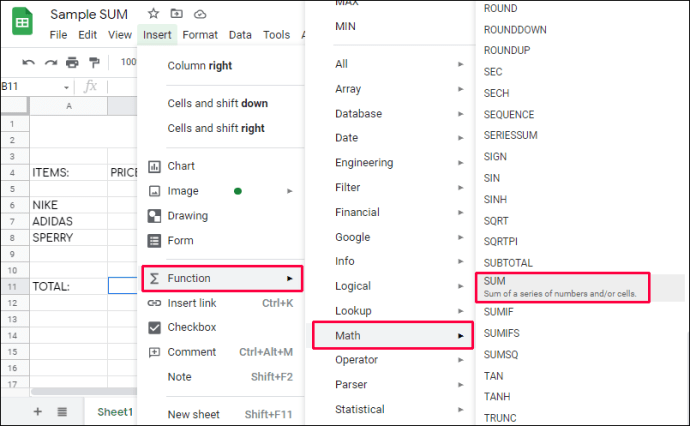
Optionally, you can choose the required function from the menu instead of typing in the formula. Follow the steps below:

1. Click any blank cell.
   
2. Click the “fx” button. It’s located at the bottom left corner of your screen in the mobile version. On the desktop version, it’s located to the right from the formatting bar.
   
3. Select “FUNCTION” from the menu, then “MATH” and select “SUM.”
   
4. To sum certain cells located in a random order, click on each one. You’ll see the cell numbers appear in your formula.
   
5. To sum a range of cells – for instance, in the same row – type in the number of the first cell or click it.
   
6. Type in the “:” symbol without pressing space and enter the number of the last cell in your range or click it. Optionally, you can click and hold an edge of the frame around the first selected cell. Then, hold and drag it to select the range.
   
7. Hit the “Enter” key or click the green checkmark to the right from the formula bar. Your sum result will appear in the selected cell.
   

In this section, we’ll answer more questions about using the SUM function in Google Sheets.

To SUM It Up

Hopefully, our guide has helped you find the sum of values in a row in Google Sheets. When used smartly, this simple function can free you from unnecessary hassle. Follow our tips to select required values quicker and keep in mind the notes. Correct utilization of the SUM function eliminates the risk of a human mistake in calculations and ensures that the sum is updated accordingly to change in values.

Do you find the SUM function better implemented in Google Sheets or MS Excel? Share your opinions in the comments section below.

Adblock test (Why?)

Original page link

Best Cool Tech Gadgets

Top favorite technology gadgets